Regularization and Generalization in Deep Learning

About Regularization and Generalization

Regularization is one of the most important concepts in machine learning. In mathematics and statistics, finance, computer science, machine learning and inverse problems regularization is the process of adding information to solve an ill-posed problem. In the context of machine learning optimization problems, it applies a modification to the objective functions to reduce generalization error of the learning model even at the cost of increased training error. Generalization refers to the capability of a trained model to make the right predictions when faced with unknown input data during its operational life.

In the rest of this article, we try to gain an intuitive understanding of the mathematical basis of regularization theory for inverse problems and its application to improve the generalization performance of learning algorithms. I have included some mathematical content to emphasize that, there is sufficiently strong mathematical foundations that support machine learning algorithms. Very often it is easy to subscribe to these algorithms with available APIs without having any understanding of their mathematical basis. However, this knowledge is shallow. Hope readers will appreciate that comment.

Forward and Inverse problems in modelling

Analysis in science and engineering involves developing models of physical systems. These models can be used to predict how the systems react to its environment with an excitation at the input (which is the cause) to produce the response at the output (which is the effect).

Figure-1

This method of analysing and predicting a system behaviour is called a direct or forward problem.

Forward or Direct problems

A direct or a forward problem starts with a cause, as an example a pattern x_n ∈ R^I  from the input data space X which is I - dimensional when transformed through a system results in a desired output y_n ∈ R^d  which is an observable effect in the output data space Y with d - dimensions.

Consider the dataset X = {x₁, x_2, ....., x_N}   and correspondingly Y = {y₁, y_2, ....., y_N}. It is assumed that X and Y are in linear vector spaces. The mapping

is a forward transformation represented by a function f(x_n), where n = 1, 2, …., N. This means

 

Forward transformation function f(.) may either be linear or non-linear. The goal is to predict the desired unique output given the input data using an appropriate physical or mathematical model that represents the transformation. Once the model is determined it is used to predict the effect given the cause.

Figure-2

In general forward transformations are represented by an operator A which may be either a matrix, a differential equation or even a transformation of a cause into an effect that can be measured as in an instrument (e.g., thermal expansion of material resulting in an indication for temperature, voltage across a piezo-electric cell for pressure, displacement of a needle for speed etc. In our context we continue to use “f ” that operates on “x” to denote such transformations to “y”.

Figure-3

Forward problems are not always well-posed, but in most cases they are. Well-posed problems have unique solutions exist that are insensitive to small perturbations in input data (can be due to noise) or in the initial values. 

Figure-4

Insensitiveness to small changes in data and other conditions indicates to the stability of the solution.

Figure-5

The figure above illustrates an unstable situation where small changes in the data causes different solutions which are the blue and pink coloured responses.

Forward-Inverse problems

A forward problem indicates the existence of a “inverse problem”. For forward inverse or in short called inverse problems, the task is to recover the cause given the effect. In that sense they are antonyms to forward problems.

Figure-6 

Very often all characteristics and parameters of the physical system are not known. It is therefore required to infer these characteristics from known responses (e.g., the RLC circuit output voltage “e₀” ) of the system.

Consider the problem of inferring the animal class that caused the observed footprints in the figure below. These types of problems are known as inverse problems.

Figure-7 

Inverse problems are concerned with determining the causes x_n of a desired effect or an observed effect y_n even though the physical properties of the model are unknown. In other words the inverse problem tries to infer the inputs by observing the outputs. This is similar to the situation that we observe the symptoms (effects) and try to answer “What is disease (cause) that resulted in the symptom?” or “What is question to which the answer is Thiruvanthapuram?” 

Solving these problems amount to identifying inverse mapping which can be expressed as 

 

These problems are very active in the field of research in applied sciences such as signal processing, machine learning, computer vision, astronomy, solutions of differential equations, various areas of engineering, etc.

Figure-8 

In mathematics the existence of inverse of function is an important property. The inverse mapping from space Y to space X exists if-and-only-if the forward mapping from X to Y is “one-to-one” and “onto”. Such mappings are said to be both injective and surjective, hence bijective.

Well posed and ill posed problems

Hadamard’s Definition of well posed problems.

The concept of a well-posed problem is due to the French mathematician Jacques. Hadamard (1923), who took the point of view that every mathematical modelling problem corresponding to some physical or technological phenomenon must be well-posed.

 Figure-9 

Hadamard postulated that inverse problems are well posed if their solutions satisfy three conditions.

• The solutions exist. (i.e., for every f (x_n) there exists a desired output y_n.). 
• The solutions are unique such that (f (x_n) ≠ f (x_j) for all n ≠ j). 
• The solution is continuously dependent on the input. (Small changes in the input will only lead to small changes in output.)

This also means that a well-posed problem is always well defined, unambiguous (easily identifiable), the solution is a single correct answer, and free from internal contradictions. 

Figure-10

Another definition according to Nashed (1987) a problem is well-posed if the set of data/observations is a closed set (i.e., the range of forward mapping is closed). In the following discussion we consider Hadamard’s definition.

The following figure illustrates the notion of ill posed problems.

Figure-11

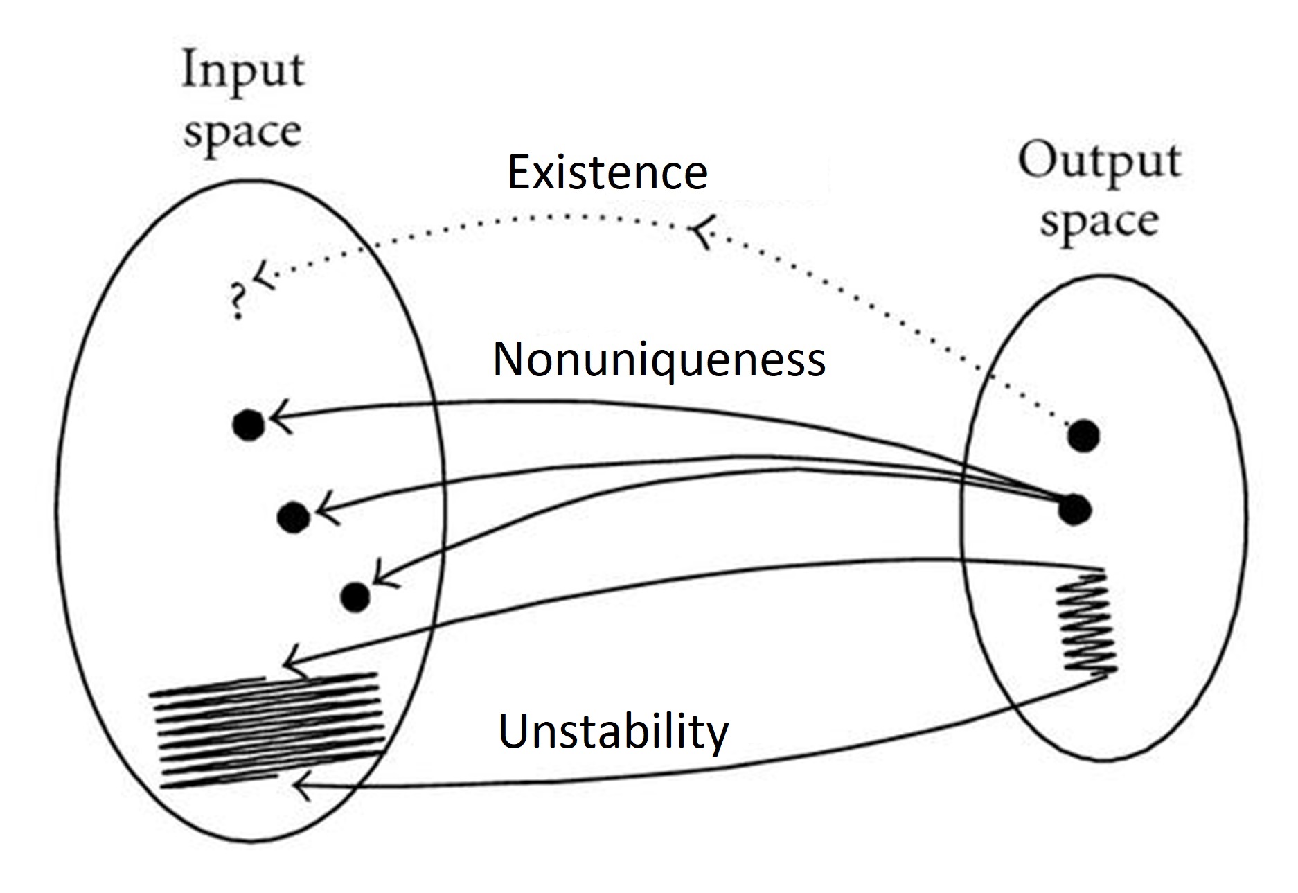
It can be seen when the output space is mapped to input space small changes in output space Y can  result in large fluctuations and undesired oscillations in the input space X causing instability.

Ill-posed problems

If any of the conditions according to Hadamard’s definition is not satisfied, the problem is ill posed. This statement holds true in general for inverse problems (and could be used as a definition). 

A broad class of the so-called inverse problems arise in physics, technology and other branches of science. In particular problems of data processing of physical experiments belongs to the class of ill-posed problems.

Ill-posed problems in purchase decisions

Figure-12 

The ill-posed inverse problem is related to solving for “x” given “y”, when “f ^-1” may not even exist or is not continuous. 

If the stability condition is violated, the numerical solution of the inverse problem by standard methods is difficult and often yields instability even if the data are exact (since any numerical method has internal errors acting like noise). 

Therefore, special techniques, the so-called regularization methods must be used to obtain a stable approximation of the solution. The appropriate construction and analysis of regularization methods and subsequently (or simultaneously) of numerical schemes is the major issue in the solution of inverse problems. 

Without regularization and without further information, the error between the exact and noisy solutions can be arbitrarily large, even if the noise is arbitrarily small. 

Inverse problems and regularization 

Inverse problem can be abstractly stated as follows: 

Given “f(.)” and “y” determine “x”, when the true solution denoted by 

 

may not exist. 

We denote the unknown solution with superscript x^† which is a minimum norm solution. The difficulty of the solution is such that even if  f ^-1(y) exists it might not be computable. 

Usually, we do not have the exact data but only the noisy data 

 

where the magnitude of

Regularization as a method to solve ill-posed inverse problems 

Regularization is applied to approximate the inverse of forward function f ^-1 by a family of stable regularization operators R_α where α being the regularization parameter. Stability is achieved by reducing the effect of noise amplification. 

The problem can be restated as 

and 

 

R_α is a continuous approximation of f ^-1.

Since the observed output data y contains random noise (δ), then the estimate of input data by observing the output data is computed as 

  

and the total error 

i.e.,

total error = data error + approximation error.

All terms both right and left hand sides are error norms. The parameter α controls the effect of regularization. When α is small, R_α is a good approximation of f ^-1, but not stable. When α is large, R_α is a bad approximation, but stable. The trade-off between stability and approximation as function of the positive parameter α is shown in following figure.

Figure-13 

The Tikhonov functional 

In the next few paragraphs, we only discuss the regularization theory proposed by Tikhonov (1963) and his colleagues for linear mappings between input space X to output space Y. Tikhonov’s method for nonlinear mapping and other regularization methods are beyond the scope of this article. 

Tikhonov’s method has been used effectively for machine learning problems and is closely related to support vector machines. The basic idea by Tikhonov et.al., is to stabilize the solution by means of an auxiliary nonnegative functional that embeds prior information about the solution. This prior information assumes that the input-output mapping is smooth. Tikhonov’s regularization theory replaces the standard squared error minimization methods with minimization of a regularization risk functional that comprises of two terms. 

This functional (a functional is function of another function that performs a linear mapping from a vector space to the real line) is defined as

where α is a positive real number called the regularization (penalty) parameter and J_α(x) is called the Tikhonov functional. The notation E_N stands for the expected value over the dataset comprising of N samples of the squared terms. 

The space of this mapping is a linear vector space of functions on which the norm is defined and is typically a Hilbert space. (For those who are not familiar vector space and functional analysis do not bother about this new term, it enough to know that Hilbert space is a generalization of Euclidean space). 

Estimating the approximation to find

is performed by minimising, optimizing the above functional in the least squared sense, i.e.,

The second term α||x||² is called the smoothness term or a stabilizer because it stabilizes the solution of the inverse problem.   If α is correctly chosen then solution converges

 and

Addition of regularization term can encode prior knowledge of x which helps to convert the ill-posed inverse problem to a well-posed one. Regularization coefficient α controls the importance of data dependent error and regularization term. Regularization parameter thus represents a trade-off between closeness to data and smoothness. The limiting values of α are 0 and ∞. With α tending to 0, the problem is unconstrained with the solution being completely determined from the training samples and is same as the standard least square error solution. With α tending to ∞, the solutions are unreliable. 

Regularization and Generalization for Machine learning and modelling 

The classical approach of modelling a linear or nonlinear transformation by a matrix or a differential equation or a measurement process etc, is not suitable for all applications and has certain drawbacks. Such analytical models are not always complete. Solving a partial differential equation with big data is computationally complex can take very long amount of time to achieve a solution. 

Machine learning models are data driven algorithms which are not explicitly programmed. They perform learning from large amount of data in most cases which are typically high dimensional to make inference, predictions and take decisions. They learn to infer an underlying mapping from an input data space X to an output data space Y. Machine learning models learn the input output relationships from a given finite sized dataset that is expected to represent a much larger collection of available data. That means the learned model must be capable to generalize or make the right estimates or prediction with data samples not seen during training. 

Deep Learning and Ill-posed Inverse problems

 

Machine learning models offer an alternative to analytical approaches by learning to infer from the given dataset {(x₁,y₁), (x₂,y₂), ……,(x_N, y_N)}. The problem of learning from examples is an example of inverse problem. These models learn to infer from a given finite sized available dataset which is partitioned for training and testing. The main goal is to generalize well on unseen data which is much larger in size than the dataset. 

Figure-14

A machine learning model uses the set of training samples to approximate a function (predictor) called a hypothesis that maps input data variable to their corresponding targeted output data variables (responses). The learning algorithm governs the learning process with a set of well-defined rules.  

These algorithms must choose a hypothesis h from a set of predictors called the hypothesis space H such that its error over the available dataset is minimized.  Once trained the model is expected to predict correctly even with unseen input data. Learning to produce the right response for any random input data from a finite set of samples is an inductive process which is an ill-posed problem. 

This problem is not solvable without making additional assumptions to make it well defined. By restricting the learner to choose a predictor from space H, we bias it towards a particular set of predictors. The choice of the restriction of predictor hypothesis space H is done based on some prior knowledge about the problem to be learned. This method of selecting the optimal h from restricted set of predictors by observing a finite set training data results in the phenomenon called inductive bias (a.k.a. learning bias).  

Regularization theory proposed for ill-posed inverse problems can be easily adapted to learning models. The work of Vapnik and his colleagues in statistical learning theory to control the model complexity to arrive at optimal solutions is the basis of applying regularization methods to ill-posed problems. The solutions correspond to a target function that performs the mapping between input data and output data. Regularized solutions in learning problems provide stable approximate solutions and gives continuous estimates of the ill-posed problems.  

A machine learning model uses a set of training samples to approximate a function (predictor) called a hypothesis that maps input data variable to their corresponding targeted output data variables (responses). The prescribed set of well-defined rules which governs the learning process is called a learning algorithm. 

Advantage of Deep Learning for modelling physical systems

Deep artificial neural network models with large number of hidden layers are universal function approximators. An ANN is an abstract machine which creates a non-linear mapping between an I-dimensional input data space and a d-dimension output space. 

Figure-15 

This non-linear mapping is captured in the weight and bias parameters of the network during the learning process of a neural network. Learning methods are essentially iterative gradient descent based methods. The "art" of training a neural network is to control the learning such that the resulting mapping is robust to noise or errors in the data. 

The optimization algorithm is typically based on back-propagation which find weights and bias parameters that minimize the error metric between computed output values and the correct output values in an iterative manner.

During training, the back-propagation algorithm iteratively adds a delta value (which can be positive or negative) to each weight and bias. The weight/bias delta is a fraction controlled by the learning rate (usually represented by η) of the weight gradient. The weight gradient is the calculus derivative of the error function. 

Due to availability powerful parallel computing facility deep learning algorithms can be efficiently implemented. Their performance improves with bigger amounts of data and can capture multiscale information. The optimization of the functional J_α(x) is achieved by iterative optimization methods. These factors have enabled solutions involving practical data that are traditionally difficult with analytical methods, and lead to faster and more effective algorithms. 

Figure-16 

These methods attempt to achieve a stable approximate solution to the exact solution of

as shown in the following figure for an image restoration problem

Figure-17 

Why Regularization is required in deep  learning 

An overly complex model can overfit any given dataset. Minimization of the cost function in the least squared sense can result in unstable solutions.  Regularization methods in deep learning helps to achieve the following objectives. 

• Minimize model complexity by punishing the weight parameters of the model.
• Eliminate overfitting. 
• Improves generalization

Consider a cost function comprising of the standard mean squared error

  

(For brevity of notatons we consider the targeted output values of all instances are scalars therefore we replace the vector notation of output with scalar representation and the weight matrix with a vector.)

The degree of the polynomial increases as the model gets complex and can fit to all the data points in the dataset. In deep learning number of learnable parameters is often considered a measure of model complexity. Model complexity can be minimized during training by punishing the higher order weight values to move close to zero . 

Regularization thus provides a fundamental framework to solve learning problems and design learning algorithms. 

Generalization by Regularization in Deep Learning 

Generalization capability of learning models refers to their ability to make accurate predictions on unknown test data input not observed during the training process. For classical machine learning algorithms generalization performance is influenced the bias-variance dilemma. This means models that are over trained or with more than a certain complexity level tend to overfit on the training data perform poorly on test data. Similarly  a model which is not trained enough or without sufficient complexity will underfit.  To improve generalization by minimizing overfitting we apply an explicit regularization term to impose an additional cost for model complexity which effectively reduce complexity level. 

In any machine learning inductive bias induces some sort of capacity control that restricts the predictors to be “simple”, which in turn allows for generalization. The success of simple model that learned to fit on the training data depends on how well the model generalizes on real data. 

An interesting characteristic of deep neural networks is its implicit regularization capability i.e., their ability to generalize well on test data even with an over capacitated architecture without explicit regularization which is contrary to the usual understanding of the bias-variance trade-off. In deep networks learning biases induced by training procedures and optimization algorithms can cause implicit regularization. 

For deep networks with implicit regularization we add explicit methods. Such regularization techniques include Ridge regression (also known as Tikhonov regularization), Lasso and Elastic net algorithms. In particular Lasso method can be used for feature selection since it forces a model to use fewer parameter coefficients. 

Methods of Weight Regularization 

An extra cost associated for larger valued weights is added to the loss function. This method of penalizing the network when weight values become more irregular is called weight regularization. Examples are L₂ regularization, L₁ regularization and L₁ - L₂ regularization. By punishing the network weights values these methods achieve model complexity reduction and improve generalization. 

L2 or Ridge Regularization 

Ridge regularization was introduced by Hoerl and Kennard. This method is the most common one and is a.k.a. weight decay regularization uses the L₂ norm for the parameter coefficients. Since the standard mean squared error function is sensitive to random errors and outliers in the data, if the weight values are not constrained, they will tend to become large valued and explode. Therefore, a ridge constraint is imposed and the new optimization problem is defined as 

We assume that the input dataset X is a standardized so that it is zero centered having unit variance and the output values from Y are also zero centered. Then the L₂ cost function or the L₂ Penalized Residual Sum of Squared errors (PRSS) can be written in terms of modified cost function that includes the additional regularization term and is expressed as 

 

Or

  

where I is the dimensionality of the input data feature vector x, y a scalar target and N is number of data sample available. 

The first term measures the discrepancy between the predicted output and the true label values. The α value in the second term controls the strength of the regularization. 

The weight update equation is

 

L₂ regularization has an advantage, since the cost function includes quadratic term, minimizing the function w.r.t. the weight values is a convex optimization problem has therefore a unique solution. It thus has a closed form solution. 

The selection of α value controls the shrinkage of the weight values. As α → 0, the cost function reduces to the original residual sum of squared errors. As α → ∞, parameter values → 0. The optimal value of α is chosen such that it minimizes the expected prediction error.  The L2 method does not force any parameter values and therefore feature data variables to be zero, however it selectively assigns more importance to those features which has more variance (more information) useful to minimize the prediction error performance. It shrinks the weight coefficients of low variance feature variables. This method is good for high dimensional dataset if all features are considered important.

Figure-18 

L₂ regularization is highly sensitive to multi-colinearity in data, i.e., when multiple two or more predictor variables in data exhibit linear dependence and lack independence. Then least squared estimates of the estimates of the weight coefficients become extremely sensitive to random errors in the data. 

Figure shows the geometric interpretation of L₂ method. The objective is to minimize the cost function under the constraint that is to stay within the gray-shaded ball. The elliptical contours represent equal valued unregularized cost function values. The gray shaded ball is the region of equal valued L2 regularized functions represented by circles. The optimal set of weight values are obtained by solving the constrained optimization problem. The solution is shown at the intersection of the region with minimal cost function. The penalty term is proportionate to the squared L₂ norm of model parameters. 

L₁ Regularization or Lasso regularization

This method was introduced Tibshirani in 1996. The optimization problem is defined as 

Hence the cost function can be written as

The weight update equation is

The gradient is defined as

When w_i is negative adding α will force it to more positive and closer to zero and vice-versa. This change in weight values can result in the lesser significant feature values being removed from the weight update equation.  

Unlike the Ridge method the Lasso method can penalize weight coefficients for features and force them to zero. Hence it can be used for feature selection by selecting one variable when there are a set of highly correlated feature variables and ignore the other correlated ones. It thus enables feature size reduction and offers a sparse solution when the feature dimensionality is high. 

A drawback for Lasso is used when feature dimensionality “ I ” is large and number of training samples “ N ” is relatively less. In such cases where N > I, the method selects only “ N ” feature variables. The Lasso method selection of feature is highly dependent on dataset. 

Figure-19 

The L1-regularization method is similar to L2 regularization. The model parameters are penalized by its own absolute weight coefficients within the constraints formed by the straight edges. Figure also illustrates how L₁ method induces sparsity. The gray shaded square is region of equal valued L1 regularized functions represented by the edges. 

Elastic net 

Each of the above regularization technique offers advantages and disadvantages for certain use cases.  The Lasso method helps to reduce the feature variables, the Ridge has the advantage that it has unique optimal (minimal) solution. Elastic net combines these two methods to include both the advantages.  

The method is to minimize the following cost function which is defined as

Or

The second order (quadratic) penalty term makes the cost function strongly convex. This results in a unique minimum solution. Both Ridge and Lasso methods can be considered special cases of Elastic net.

 

The parameter 𝜆 is called the mixing coefficient. For Lasso 𝜆 = 1 and for Ridge 𝜆 = 0. For 𝜆 > 0, minimization of the cost function is always a convex optimization problem.

 

In the naive implementation of elastic net method finds an optimal set of weight values in a two-stage method. First the ridge coefficients are determined and then the {\displaystyle \lambda _{2}}a lasso type shrinkage performed. This two-step method causes double shrinkage of weight coefficients. The prediction capability of the model decreases due to increased bias. To compensate for this the estimated coefficients can be multiplied by (1+ α₂).

Figure-20 

The above figure shows a comparison between the above methods. Two-dimensional contour plots of the ridge penalty; lasso penalty and the elastic net penalty with α = 0.5. Vertices are point of singularities. For lasso the edges are straight lines. For both ridge and elastic net, the edges are strictly convex; for elastic net, the strength of convexity varies with α

 

Other methods to tackle overfit in learning models

 

Dropout: This method is used for deep artificial neural network models. While training during each update cycle, a neuron output is active only with a certain probability “p”. Each dropout layer chooses a set of random units with probability “1-p” and set their outputs to zero and the synaptic weights are not updated.   The random dropout of nodes is performed only during training and not done during testing.

Figure-21

 

Batch Normalization: It is general practice to initialize the network parameters with zero mean and unit variance. As training progresses the set of weight values loses this property.   Using batch normalization of layer weights re-establishes this property. It also helps to reduce the need for dropout.

 

Combining Multiple Learners (Ensemble method)

According to the “No Free Lunch Theorem” there is no single learning algorithm that is always the most accurate in any problem domain. The usual approach is to try many and choose the one that performs the best on a separate validation. The simplest way to combine multiple learners corresponds to taking a linear combination of the L base learners to reduce the problem of overfit and reduce variance. Important characteristics of base learners are 

a) Diversity- independence and lack of correlation

b) Accuracy and

c) Computational speed. 

There are two different ways the multiple base-learners that complement each other are combined to generate the final output.

Multi-expert Combination 

Multi-expert combination methods have base-learners that work in parallel. Examples are voting and stacking.

For class predictions a majority vote is considered and for regression averaged output is used. These learners use a bagging scheme whereby the L different and independent base learners are trained over slightly L different training sets which are randomly chosen from the set with replacement. Bagging is a short form for bootstrap aggregation. Random Forest Classifiers are examples of ensemble learning that use bagging.

Figure-22 

Model stacking is an efficient ensemble method in which the predictions, generated by using various machine learning algorithms, are used as inputs in a second-layer learning algorithm. This second-layer algorithm is trained to optimally combine the model predictions to form a new set of predictions. For example, when linear regression is used as second-level/layer modelling, it estimates these weights by minimizing the least square errors. However, the second-layer modeling is not restricted to only linear models; the relationship between the predictors can be more complex, opening the door to employing other machine learning algorithms.

Figure-23

Multistage Combination 

Multistage combination methods use a serial approach where the next base-learner is trained with or tested on only the instances where the previous base-learners are not accurate enough. The idea is that the leaners are sorted in increasing complexity so that a strong and complex learner is not used (or its complex representation is not extracted) unless the preceding simpler weak learners are not confident. Boosting uses simple base models and tries to “boost” their aggregate complexity. Unlike bagging methods where individual learners are independent, boosting processes are sequential and iterative. Adaboost (AdaBoost is short for Adaptive Boosting and is a very popular boosting technique) and Gradient Boosting machines are examples of this type (XGBoost is one of the fastest implementations of gradient boosted trees.).

Figure-24

 

Early Stopping: According to G. Hinton “early stopping is free-lunch”. During validation the model performance is monitored and number training epochs when no further improvement is observed. In the figure below the number of training epochs for the deep learning model can be limited to 7 so that the validation error is minimizes even though the training loss seems continues to decrease when the epochs are continued.

Figure-25

 

 

Data Augmentation

 

Data augmentation for training is a widely used technique to improve generalization performance of machine learning models particularly in image and natural language processing related datasets.

 

Unlike traditional models the performance of deep learning architectures consistently improves with increased dataset sizes. However datasets with large sizes are not easily obtainable.  Hence techniques to synthesize additional data sample by manipulating the original one is an easy and cheaper alternative. Figure below is block diagram that involves both human and deterministic sequence of transformations on the original dataset to augment. Data augmentation may be done such that it does not exceed an upper bound that can result in considerable difference between the original set and the enhanced one, causing adversarial effect in model performance. Generative adversarial networks are being utilized for automatic data enhancement.

Figure-26

 

Adding random noise in feature data during training is an augmentation strategy. Another method is to add noise in network weights to make the model insensitive to small weight changes.

 

 

References

1. Heinz W. Engl, Martin Hanke, Andreas Neubauer, “Regularization of Inverse Problems”, Springer 
2. Ajay Verma, Michael W. Oppenheimer, David B. Doman, On-Line Adaptive Estimation and Trajectory Reshaping, September 2005, DOI: 10.2514/6.2005-6436 
3. Kshitij Tayal, Chieh-Hsin Lai, Vipin Kumar, Ju Sun, Inverse Problems, Deep Learning, and Symmetry Breaking,  arXiv:2003.09077v1 [cs.LG]  
4. Lucas A., Michael Iliadis, R. Molina, A. Katsaggelos, Using Deep Neural Networks for Inverse Problems in Imaging: Beyond Analytical Methods,Published in IEEE Signal Processing Magazine 2018 
5. Connor Shorten &  Taghi M. Khoshgoftaar , “A survey on Image Data Augmentation for Deep Learning”, Journal of Big Data volume 6, Article number: 60 (2019) 
6. Aristide Baratin, Thomas George, César Laurent, R Devon Hjelm,
7. Guillaume Lajoie, Pascal Vincent, Simon Lacoste-Julien, “Implicit Regularization via Neural Feature Alignment”, arXiv:2008.00938v2 [cs.LG] 28 Oct 2020
8. Gitta Kutyniok, Solving Mathematical “Problems by Deep Learning:
9. Inverse Problems”, Woudschoten Conference Zeist, The Netherlands, October 9{11, 2019
10. Sargur Srihari, “Regularization in Neural Networks”, buffalo.edu
11. Ernesto De Vito, Umberto De Giovannini, Lorenzo Rosasco, Francesca Odone. “Learning from Examples as an Inverse Problem.”, Article in Journal of Machine Learning Research · May 2005
12. Hyeontae Jo, Hwijae Son,  and Hyung Ju Hwang, Eun Heui Kim,  “Deep Neural Network Approach to, Forward-Inverse problems”,  Networks and Heterogeneous media, American Institute of Mathematical Sciences, Volume 15, Number 2, June 2020 pp. 247
13. Karl-Heinz Ilk, “On the Regularization of Ill-Posed Problems” , researchgate.net/publication/234423030
14. Devis Tuia, Remi Flamary, Michel Barlaud, To Be or Not To Be Convex? A Study on Regularization in Hyperspectral Image Classification, Published in: 2015 IEEE International Geoscience and Remote Sensing Symposium (IGARSS),  DOI: 10.1109/IGARSS.2015.7326942
15. https://statweb.stanford.edu/~owen/courses/305a/Rudyregularization.pdf
16. https://en.wikipedia.org/wiki/Machine_learning#Training_models
17. http://www.statistics4u.com/fundstat_eng/cc_ann_recurrentnet.html
18. http://www.kjdaun.uwaterloo.ca/research/inverse.html
19. https://in.mathworks.com/discovery/regularization.html
20. http://d2l.ai/chapter_multilayer-perceptrons/weight-decay.html
21. https://blog.datadive.net/selecting-good-features-part-ii-linear-models-and-regularization/ 
22. https://www.coursera.org/lecture/ml-regression/can-we-use-regularization-for-feature-selection-0FyEi
23. https://www.cs.ubc.ca/~murphyk/Teaching/CS540-Fall08/L13.pdf
24. https://ml-cheatsheet.readthedocs.io/en/latest/regularization.html
25. https://www.youtube.com/watch?v=MiFQt5CYM4Y
26. https://www.youtube.com/watch?v=dYMCwxgl3vk

Image Credits

Figure-1: slideshare.net

Figure-4: Reference 2

Figure-5: Reference 2

Figure-7: shutterstock.com/508591663.jpg

Figure-9: mathsisfun.com

Figure-10: siltanen-research.net

Figure-11: static-01.hindawi.com

Figure-12: kjdaun.uwaterloo.ca

Figure-13:

Figure-14: guru99.com

Figure-15:

Figure-16: groundai.com

Figure-17: Reference 4

Figure-18: rasbt.github.io

Figure-19: rasbt.github.io

Figure-20: drek4537l1klr.cloudfront.net

Figure-21: cs.toronto.edu

Figure-22: researchgate.net

Figure-23: blogs.sas.com

Figure-24: miro.medium.com

Figure-25: Reference 6

Figure-26: ai.stanford.edu