Linear Algebra for AI and ML

Linear algebra and applied mathematics

Applied mathematics rests on two central pillars: calculus and linear algebra. Calculus has its roots in the laws of Newtonian physics. Linear algebra arises from the need to solve simple systems of linear algebraic equations. Linear algebra plays profound roles in both applied and theoretical mathematics, as well as in all of science and engineering, including computer science, data analysis and machine learning, imaging and signal processing, probability and statistics, economics, numerical analysis, mathematical biology, and many other disciplines. Knowledge in both calculus and linear algebra is an essential prerequisite for a successful career in science, technology, engineering, statistics, data science and mathematics.

What is Linear Algebra

Linear algebra is a branch of mathematics that describes linear systems with linear equations and linear functions and deals with their solutions. An equation is linear if it does not have any term in it with exponents greater than one. A system is linear if it satisfies the conditions of superposition and homogeneity. A system of linear equations (or linear system) is a collection of one or more linear equations involving the same variables (wikipedia).  

Linear algebra is the study of linear combinations, including vector spaces, lines and planes, and the mappings that are required to perform the linear transformations. It deals with linear equations and their representations in vector spaces and through matrices. It helps to understand their underlying structure of linear systems.

It is used to model of a large variety of natural phenomena and allows efficient computation with such models.  A system of linear equations model real world systems with linear characteristics. They occur when we have two or more linear equations working together. Such equations are used to solve problems in various fields such as Economics, Engineering, Physics, Chemistry, Transportation and Logistics, Investment forecasting and several more. Nonlinear systems are often dealt by linear algebra with first-order approximations.  

Let us assume there are two equations and two unknowns. 

3 = - y – 2x

2 = y + 3x

Figure-1:

This system can be solved in many ways. One method is by subtracting the second one from the first one, then we get

-5 = -5x, i.e., x = 1

The value of the unknown x is computed. The solution to the system found by substituting x = 1 and we get y = -1, where the lines intersect.  

In the above system there are only two equations and two unknown variables. When the number of equations is same as the number of unknown variables a solution is possible though not guaranteed. There are three possible situations.

1. No solutions exists, then the equations are inconsistent. 
2. Only one solution exits. 
3. Infinite number of solutions exists.

When either one solution or infinite solutions exists the system of equations is consistent.

Figure-2:

Linear equations in 2D space define lines, similarly those in 3D space define planes.

Figure-3:

Finding solutions to 3 variable linear equations means finding the intersections of planes. For 3 variable system of equations there are the following possible cases of solutions.

1. All the three planes intersect at a point. Then there is a unique solution.
2. The three planes intersect or coincide along a line on a plane, in which case there are infinite solutions.
3. No intersection at all or they intersect in pairs. In this case there is no solution. 

In the following figures starting from the top left hand side Figures 1, 3, and  4 donot have solutions. Figure 2 has infinite solutions, and Figure 5 has a unique solution

Figure-4:

Systems that have a single solution are those for which the ordered triple (x,y,z) defines a point that is the intersection of three planes in space. Systems that have an infinite number of solutions are those which, for which the solutions represent a line or coincident plane that serves as the intersection of three planes in space. Systems that have no solution are those represented by three planes with no point or line in common.

Equations with number of variables n > 3 dimensions define hyperplanes. As the number of variable and equations increase solutions become more complicated. 

All linear systems while outwardly different are truly similar at their core. Basic mathematical principles such as linear superposition, the interplay between homogeneous and inhomogeneous systems, the Fredholm alternative characterizing solvability, orthogonality, positive definiteness and minimization principles, eigen values and singular values, and linear iteration, to name but a few, reoccur in many ostensibly unrelated contexts.

Outside of algebra, a big part of analysis called functional analysis, is actually the infinite-dimensional version of linear algebra. In infinite dimension, most of the finite-dimension theorems break down in a very interesting way; some of our intuition is preserved, but most of it breaks down. Of course, none of the algebraic intuition goes away, but most of the analytic part does; closed balls are never compact, norms are not always equivalent, and the structure of the space changes a lot depending on the norm you use. Hence even for someone studying analysis, understanding linear algebra is vital.  Linear algebra has its use also in abstract algebra.

Calculus and Linear Algebra

The term “linear” refers not just to only linear algebraic equations, but also to linear differential equations, both ordinary and partial, linear boundary value problems, linear integral equations, linear iterative systems, linear control systems, and so on. 

Linear Algebra and Calculus are two fundamental areas of mathematics that are interconnected in many ways. Calculus deals with functions and their derivatives, while linear algebra involves operations on numbers and variables.

 

Differential calculus and LA.

The derivative of a function at a point is the best linear approximation to the function near that point. In optimization problems it is often required to find maxima or minima of functions by setting derivatives equal to zero. Such problems can be expressed in terms of linear algebra.

L.A. is used to deal with problems in multivariate calculus, where concepts like gradients, Jacobians and Hessians which are vectors and matrices of first and second derivatives respectively. Systems of linear differential equations can be solved using eigenvalues and eigenvectors, concepts from linear algebra.

 Matrix Calculus and Linear Algebra

The method of doing multivariable calculus is called Matrix Calculus. Matrix calculus deals with derivatives and integrals of multivariate functions (functions of multiple variables). It allows us to write the partial derivatives of such functions as a vector or a matrix that can be treated as a single entity. This greatly simplifies some common mathematical operations such as finding the maximum or minimum of a multivariate function. In essence, Matrix Calculus can be viewed as an extension of Linear Algebra to multivariate data and functions. It is a fundamental tool for understanding and solving problems in machine learning and data science. Multivariable calculus called matrix calculus greatly simplifies finding the maximum and minimum of a multivariate function and solving linear differential equations.

 Integral calculus and LA.

The concept of linear transformations, a key topic in linear algebra, is also important in integral calculus. For instance, the Fourier Transform, which is used extensively in integral calculus, is a type of linear transformation. Numerical methods for approximating integrals often use concepts from linear algebra. For example, the method of least squares, which is used to fit a function to data points, is a problem in both integral calculus and linear algebra. In integral calculus, functions can be treated as vectors in function spaces.

Linear Algebra the Mathematics of Data

In machine learning and data science application a dataset with real valued variables can contain hundreds of variables in which case manual solutions becomes impossible. Solutions will therefore require usage of large matrices and algorithms implemented with computers.

Linear algebra is a field of mathematics that could be called the mathematics of data. Modern statistics uses both the notation and tools of linear algebra to describe the tools and techniques of statistical methods. As the mathematics of data, linear algebra is therefore essential for understanding the theory behind Machine Learning, especially for Deep Learning. 

Matrix Factorization

Matrix factorization is a key tool in linear algebra and used widely as an element of many more complex operations such as matrix inversion, Singular-Value Decomposition and Principal Component Analysis (used for data reduction and dimensionality reduction), machine learning (least squares), implementation of various machine learning algorithms viz. clustering, recommender systems, collaborative filtering etc.

Linear Least Squares

The complexity of solutions increases as number of unknown variable and number of equations increase. A single solution may not exist and lines or planes will not fit the data perfectly. Solutions are not possible without some error. Under these situations solutions of linear system of equations rely on optimization (minimization or maximization) methods. A method often adopted is minimization of squared errors called least squares solutions. Least squares solution is used for linear regression models and wide range of machine learning algorithms. Linear least squares solutions can be solved efficiently on computers with matrix factorization.

The basic entities or objects of Linear Algebra - Scalars, Vectors, Matrices and Tensors are the basic mathematical objects extensively used in fields like machine learning and data sciences.

Scalar

A scalar is fully defined by its numerical value or its magnitude which is a single element and therefore it one-dimensional and has no direction. A scalar field F has a particular value at every point in the one dimensional space e.g., Rⁿ where n = 1.

Vector

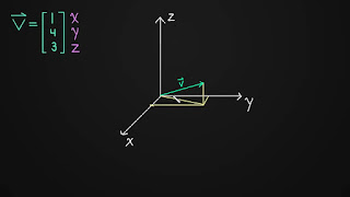
A vector has more than one element i.e., n > 1 and hence is n dimensional element in a vector space. Vectors can be grouped to form a vector space V e.g., R³. An n dimensional vector represents a point with magnitude and direction in an n dimensional space. Real valued spaces with n dimensions are denoted by Rⁿ, correspondingly complex values denoted by Cⁿ.

Figure-5:

Vectors were introduced in physics to deal with magnitudes of forces acting in specific directions and in geometry as elements in Euclidean space before the conceptualization of vector spaces. In linear algebra vectors are a list of numbers which identify a point in a vector space, each number being a component corresponding to its dimension.

Vector space
A vector space is a nonempty set V of vectors on which two operations vector addition and scalar multiplications are defined, if it satisfies the following properties. 

• Scaling or scalar multiplication of  vectors i.e., f(αv) = αf(v). 
• Superposition i.e., for any two vectors v and u,  f(v + u) = f(v) + f(u)

A vector space can be divided into subspaces. If W is a subset of V which satisfies all operations in V, it is called a subspace of V e.g., R² is subspace of R³. A finite n – dimensional vector space is a set or collection of n-dimensional vectors which can added/subtracted together and scaled or multiplied by numbers which are called scalars.

Figure-6:

Vector spaces a.k.a. linear spaces are characterized by its dimensions. They are useful to deal with linear systems of equations. Vector spaces arise in many different areas of algebra such as group theory, ring theory, module theory, representation theory, Galois theory, and much more. Understanding the tools of linear algebra gives one the ability to understand those theories better. Some theorems of linear algebra require also an understanding of those theories; they are linked in many different intrinsic ways.

Key operations that can be performed with vectors are

1.  Addition and Subtraction u + v, u – v, etc. 
2. Convex combinations such as αu + βv, α and β such that α + β =1. Dot product of two vectors u.v is results in a scalar value. 
3. Computing the angle θ between u, v where cosine(θ) = u.v / (||u||.||v||). 
4. Transpose of vector u is denoted by u^T, the transpose of column vector u is a row vector and vice-versa. 
5. A row vector is also a 1D array. The inner product of u^T.v is a scalar quantity.  
6. The u^T.u is the square of its magnitude. 
7. The outer product of u.u^T  is a matrix of n x n dimension which is 2D array. 

Matrix

A matrix is a rectangular arrangement of n rows and m column vectors of n dimensions. Hence it is an n x m, 2dimensional array formed as collection of m vectors each with n dimensions. They play a central role in linear algebra. They can be used to compactly represent systems of linear equations, but they also represent linear functions (linear mappings).

Matrices are denoted by capital letters A, B, etc. An example of m x n matrix is shown below

Figure-7:

Linear systems can be represented and solved with matrix equations. Therefore linear algebra can be considered the study of linear maps or transformations on finite-dimensional vector spaces.

Figure-8:

Sparse Matrices

A sparse matrix is one in which most elements are zeros. Imagine a matrix where columns represent every movie on Netflix, the rows are every Netflix user. Consider that values entered indicate how many times a user has watched that particular movie. This matrix would have tens of thousands of columns and millions of rows! However, since most users do not watch most movies, the vast majority of elements would be zero. Sparse matrices only store nonzero elements and assume all other values will be zero, leading to significant computational savings.

Key operations that can be performed with matrices

Consider U and V are two matrices and α, β are scalar.

1. Scalar multiplications αU , βV. 
2. Transpose of n x m matrix U, is U^T is an m x n matrix. 
3. The product of n x m matrix U with a m x n matrix V, is W =  UV which is an n x n matrix. 
4. The product of m x n matrix V with a n x m matrix U, is R=  VU which is an m x m matrix. 
5. If two matrices are of same dimensions the following operations can be performed.    Addition and Subtraction U + V, U – V, Element –by – element product U.*V,     Element – by – element power U.^V, Element –by – element right division U./V,     Element –by – element left division V./U

Terms related to Matrices

Dimension or order of Matrix – If a matrix has n rows and m columns, order of the matrix is n x m which is read as n by m.

Square Matrix – The matrix in which the number of rows is equal to the number of columns.

Diagonal Matrix – A matrix with all the non-diagonal elements equals 0 is called a diagonal matrix. The term usually refers to square matrices.

Upper triangular Matrix – Square matrix with all the elements below diagonal equals 0.

Lower triangular matrix – Square matrix with all the elements above the diagonal equals 0.

Scalar Matrix – Square matrix with all the diagonal elements equals some constant k.

Identity Matrix – Square matrix with all the diagonal elements equals 1 and all the non-diagonal elements equal to 0.

Column Matrix

The matrix which consists of only single column. Sometimes, it is used to represent a vector.

Row Matrix – A matrix consisting only a single row.

Trace – It is the sum of all the diagonal elements of a square matrix.

Rank of a Matrix – Let “c” be used to denote the maximum number of linearly independent column vectors  and “r” for maximum number  of linearly independent row vectors of a matrix.  Then rank of a matrix is min(r,c). A column or row vector in a matrix is linearly independent if it cannot  be expressed as a linear combination of any other column or row vectors in the matrix.

Determinant of a Matrix – Determinant is scalar value, defined only for square matrices. It is used for the analysis and solution of systems of linear equation. A square matrix with non-zero determinant is called a nonsingular matrix. A non-homogeneous system of linear equation has a unique solution iff the determinant of system matrix is nonzero. It is denoted by det(U), det U or |U|.

Minors of a matrix - The minor of a matrix exists for every element u_ij of a square matrix. It is the determinant of sub-matrix formed by ignoring the i^th row and j^th column of U. Since minors of matrix element are determinant values they have no polarity or signs. A matrix of minors is a square matrix of same order of U formed by its minors.

Cofactors of a matrix – Cofactor of matrix element is formed by including the polarity of minors. If i + j is even, cofactor of u_ij polarity is positive. If i + j is odd, cofactor polarity of u_ij, is negative. A matrix of cofactors is a square matrix of same order of U formed by its cofactors which includes the polarities.

Adjoint of a matrix – Also called the adjugate or adjunct of square matrix U is the transpose of its cofactor matrix.

Inverse of a Matrix - The inverse of matrix U is U^-1, if UU^-1 = I, where I is identity matrix. The inverse of nonsingular matrix U can be computed as 

In matrix algebra there is no division by a matrix we only multiply with matrix inverse e.g., VU^-1. It must be noticed that VU^-1 ≠ U^-1V. Not all matrices have inverses. Inverse of matrix exists only for square matrices provided their determinants are not equal to zero. If determinant equals zero, then the matrix is called singular matrix. A singular matrix is non-invertible.

Eigenvalues and Eigenvectors

Eigenvalues of a linear system of equations (a.k.a. matrix equations) are characteristic values (roots) of the matrix equation. For every nonzero eigenvalue there is an associated vector called eigenvector. The eigenmatrix of an n x n matrix A is a diagonal matrix formed by its eigenvalues. All eigenvectors are independent and orthonormal to each other. In a finite n-dimensional vector space, eigenvectors are its basis vectors. The method of decomposing a square matrix into its eigenmatrix and eigenvectors is called eigenvalue decomposition.

Matrix decomposition, also known as matrix factorization, involves describing a given matrix using its constituent elements. Eigenvalue decomposition factorizes a matrix into its eigenvalues matrix and eigenvector matrix.

Let A be a positive semi-definite matrix then its eigen-decomposition can be expressed as

where U being an orthonormal matrix (i.e., U^TU = I) and Λ being a diagonal matrix containing the eigenvalues of A. 

This factorization can be performed only by for diagonalizable matrices. It is also called spectral decomposition. If one or more eigenvalues of a  matrix are zero then its determinant is zero. In general, a matrix with complex eigenvalues is not diagonalizable. 
Consider a 2d vector x  = [x, y]^T and a matrix 2 x 2 matrix A. If the transformation of vector x performed by multiplying it with A, preserves the direction of x but scales it by a value λ 

i.e.,

Then x is an eigenvector associated with the eigenvalue λ of the matrix A. The following figures illustrates the concepts of eigenvalues and eigenvectors. 

Figure-9:

In the figure below the blue vector direction is preserved where as that of red vector has changed, this means the blue vector is an eigenvector is of the matrix that transformed the first image to the second. Therefore eigenvectors of matrix do not change its direction during a transformation by the matrix. The length of the blue arrow does not change therefore its corresponding eigenvalue is 1 (wikipedia).

Figure-10:

Eigenvalues and eigenvectors have a wide range of applications, for example in stability analysis, vibration analysis, atomic orbitals, facial recognition, and matrix diagonalization, data dimensionality reduction, data compression, multivariate statistics, quantum computing and more.

Singular Value Decomposition

Singular value decomposition is a factorization of a real or complex matrix is a generalization of eigenvalue decomposition. SVD decomposes a matrix (any size) from data space into another space. This {\displaystyle m\times n}is perhaps the most widely used matrix decomposition method. All matrices have an SVD, which makes it more stable than other methods, such as the eigen-decomposition. Eigen-decomposition method factorizes a square matrix mainly to two simple matrices. But SVD method decomposes a matrix to three simpler matrices two orthonormal matrices and one diagonal matrix. It is perhaps the most known and widely used matrix decomposition method. 

SVD helps to reduce data dimensionality by selecting the key features necessary for analysing and describing data. It may be considered a data driven generalization of the Fourier transform which maps data in a certain co-ordinate system to another co-ordinate system where the data analysis is simplified (consider the transformation a complex signal comprising of multiple frequencies in time domain to frequency domain where the individual frequencies can be easily visualized.  SVD forms the basis Principal Component Analysis (PCA) which is one of the most important data dimensionality reduction techniques. 

The singular values of a matrix M are the square roots of the eigenvalues of M*M, where * denotes the transpose or Hermitian conjugation, depending on whether M has real or complex coefficients.  When applied to a positive semi-definite matrix, the SVD is equivalent to the eigen-decomposition. If M is a rectangular matrix, its SVD decomposes it as:

 

where:

U: orthogonal matrix with (normalized) eigenvectors of the matrix MM^T (i.e., U^TU = I). The columns of U are called the left singular vectors of M.

Σ:  the diagonal matrix of the singular values, Σ = Λ^1/2 , Λ being the the diagonal matrix of the eigenvalues of matrix MM^T and of the matrix M^TM (both these matrices have the same eigenvalues). The singular values are the non-negative real values of the eigenvalues of the matrix M.

V: orthogonal matrix with (normalized) eigenvectors of the matrix M^TM (i.e., V^TV = I). The columns of V are called the right singular vectors of M.

The SVD method decomposes a matrix M into three matrices: two matrices with the singular vectors and one singular value matrix whose diagonal elements are the singular values. The method factorizes matrix M into a rotation, followed by a rescaling, followed by another rotation. The diagonal entries of the rescaling matrix are uniquely determined by the original matrix and are known as the singular values of the matrix. Singular vectors of a matrix describe the directions of its maximum action. And the corresponding singular values describe the magnitude of that action.

The following figure illustrates three steps in method of SVD applied on matrix 2 x 2 matrix M. The yellow and red vectors are the canonical basis vectors represented by M of a unit disc coloured blue. Beginning the sequence from the left top corner, these vectors are rotated by the transformation due to V^T  (in the following figure please consider  V^*  =  V^T ). They are then scaled by the diagonal matrix Σ with the singular values of σ₁ for horizontal and σ₂ for vertical directions. The scaled vectors are then further rotated due to the transformation by U.

Figure-11:

SVD is used in a wide array of applications including compressing, denoising, and data reduction and to eliminate redundancy in data. In a data set with large number of features can naturally contain redundant features. Redundant information does not serve useful purposes but will only increase computational complexity and memory requirements.

Tensors and Arrays as data

A tensor is a generalization of scalars, vectors and matrices. In machine learning tensors are used to describe the operations of mainly deep learning models. The word tensor originates from the Latin word "tendere" which means to stretch. Tensors provide a framework in physics to deal problems in elasticity, fluid mechanics and general relativity.

Figure-12:

An array is a data structure that stores a collection of homogeneous type of data in contiguous memory locations. Arrays are formed by grouping of vectors to form a dataset. Every vector or data point in the array can be easily accessed by its index and element of the array can also be extracted by its indices. Multiple dimensional arrays are arrays with three and more dimensions. Tensors are containers of Data to store different dimensions of Data for deep learning and machine learning applications. The number of axes of a tensor is called it rank.

• Scalars are Rank 0 or 0D tensor. 
• Vector or Rank 1 or 1-D Tensors. 
• Matrices or Rank 2 or 2-D. Tensor. 
• 3-D Tensor and Higher Dimensional Tensor – Rank 3 tensors are packs of Rank 2 tensors, Rank 4 tensors are packs of Rank 3 tensors and so on.

Real-World Examples of Tensors and arrays

Vectors and matrices as data

For computational requirements a vector is essentially one dimensional array. Vectors are 1D arrays that represent multiple variables. They typically have a fixed length "N". They can be considered a point in an N - dimensional space.   Therefore they are unlike lists and queues which may not have a fixed length. A vector data structure is represented in linear algebra as a mathematical vector. A set of fixed length vectors forms a matrix. A matrix is a 2D array.

Data represented adequately in a suitable format can be read by a computer. Structured data may be available in tabular form, each column representing a particular data instance or sample. The rows in the table correspond to a particular feature. The column/row representation can be swapped. Vectors, arrays and matrices are useful to deal with higher dimensional data.

Data is not always structured and is available as semi, quasi and unstructured formats. Audio signals, genomic sequences, audio, text, image, video, contents of a webpage, social media graphs, etc are examples of unstructured  data. Eighty percent of available data is unstructured. Manipulating and exploiting data for machine learning models require domain expertise and require careful engineering. In recent years, they have been put under the umbrella of data science and artificial intelligence.

Matrix as vector dataset: This is an array of vectors, where the first axis is the samples axis (sample dimensions) and the second axis is the features axis. An actuarial dataset of people, where we consider each person’s age, ZIP code, and income. Each person can be characterized as a vector of 3 values, and thus an entire dataset of 100,000 people can be stored in a 2D tensor of shape (100000, 3).

Applications in Natural Language Processing

For NLP applications a collection of words called a Bag of Words matrix are numerical representations by arrays. A term-document matrix is also a numerical matrix that describes the frequency of terms that occur in a document. These techniques are useful to store counts and frequencies or words occurring a in document, measure similarity between words and so on such that Document classification, Sentimental analysis, Semantic analysis, Language translation, Language generation, information retrieval, etc can be performed.

Time-Series Data or Sequence Data: 

Whenever sets of vector or matrix data occur in sequential order perhaps in time 3D tensors are used. Application examples are a dataset of stock prices. Every minute, we store the current price of the stock, the highest price in the past minute, and the lowest price in the past minute. Thus every minute is encoded as a 3D vector, an entire day of trading is encoded as a 2D tensor of shape (300, 3) (approximately 300 minutes in a trading day), and 200 days’ worth of data can be stored in a 3D tensor of shape (250,390, 3).

Speech and Audio Data

Speech and audios signal are temporally sequential data. These signals are sampled at fixed frequencies usually at 44.1 kHz, 48 kHz etc for audio and 8 kHz, 16k Hz, 44.1 kHz etc for speech. Sampling frequency resolutions differ as per different standards.

Figure-13:

Signal information will keep change from time to time. To achieve temporal stationarity, sequences are sampled into frames of short duration of few milliseconds. Features extracted from frames that contain qualitative, temporal, spectral information, etc. Vectors of features coefficients are extracted from these frames and stacked in sequence to form n x m matrices to represent the signals. Large collection speech and audio signal data can then be stored in 3D tensors. This data can be further used for data analysis and manipulations.

Image Data

Images typically have three dimensions: height, width, and colour depth. RGB Images has three colour channels. Grayscale Images contains only one channel.

Figure-14:

Color images are general RBG images each color representing a channel

Figure-15:

Video Data

A video can be understood as a sequence of frames, each frame being a colour image. Because each frame can be stored in a 3D tensor (height, width, colour-depth), a sequence of frames can be stored in a 4D tensor (frames, height, width, colour-depth).

Higher order Tensors

Video data set is one of the few types of real-world data for which you’ll need 5D tensors. 5D- tensors of shape (samples, frames, height, width, channels) and thus a batch of different videos can be stored in a 5D tensor of shape (samples, frames, height, width, colour-depth).

For instance, a 60-second, 144 × 256 YouTube video clip sampled at 4 frames per second would have 240 frames. A batch of four such video clips would be stored in a tensor of shape (4, 240, 144, 256, 3). Figures below illustrates tensors with various dimensions

Figure-16:

The following figure illustrates methods of slicing a multidimensional tensor

Figure-17:

 

Video data is one of the few types of real-world data for which you’ll need 5D tensors. 5D tensors of shape (samples, frames, height, width, channels) and thus a batch of different videos can be stored in a 5D tensor of shape (samples, frames, height, width, colour-depth).

For instance, a 60-second, 144 × 256 YouTube video clip sampled at 4 frames per second would have 240 frames. A batch of four such video clips would be stored in a tensor of shape (4, 240, 144, 256, 3). That’s a total of 106,168,320 values! If the data type of the tensor is float32, then each value would be stored in 32 bits, so the tensor would represent 405 MB. Heavy! Videos you encounter in real life are much lighter, because they aren’t stored in float32, and they’re typically compressed by a large factor (such as in the MPEG format).

References

Topics in Algebra 2^nd Edition,   I. N. Herstein, Wiley Student Edition

Applied linear Algebra 2^nd Edition, Peter J. Olver, Chehrzad Shakiban, Springer

Linear Algebra 2^nd Edition, Larry Smith, Springer

https://www.itl.nist.gov/div898/handbook/pmc/section5/pmc53.htm

https://personal.utdallas.edu/~herve/Abdi-SVD2007-pretty.pdf

https://www.cs.cmu.edu/~venkatg/teaching/CStheory-infoage/book-chapter-4.pdf

https://www.oreilly.com/library/view/machine-learning-with/9781491989371/ch01.html

https://mc.ai/tensors%E2%80%8A-%E2%80%8Arepresentation-of-data-in-neural-networks/

https://www.dataquest.io/blog/natural-language-processing-with-python/

Figure Credits

Figure-1: study.com

Figure-2: slideplayer.com

Figure-3: study.com

Figure-4: googleusercontent.com

Figure-5: youtube.com

Figure-6: www.ibm.com

Figure-7: wikimedia.org

Figure-8: mathworks.com

Figure-9: By Lyudmil Antonov Lantonov, commons.wikimedia.org

Figure-10: By TreyGreer, commons.wikimedia.org

Figure-11: wikimedia.org

Figure-12: A representation-of-data-in-neural-networks, mc.ai  

Figure-13: google.com

Figure-14: Linear algebra singular value decomposition, andrew.gibiansky.com

Figure-15: brohrer.github.io

Figure-16: static.javatpoint.com

Figure-17 : matlab.izmiran.ru